Understanding PopulationSim, SFT, and DPO through calculations

Population weights and model weights

A population weight says how many households or people a sampled record represents. A model weight is a numerical parameter used to compute predictions. These are different quantities despite sharing the word “weight.”

PopulationSim inputs

examples/example_test/configs/controls.csv specifies control attributes, geography, source tables, importance, and aggregation expressions. seed_households.csv and seed_persons.csv supply samples; geographic aggregate files supply targets. Household–person links determine each household’s contribution to each constraint.

Consider a fictional example. Sample A contributes one household, one person, and no children; sample B contributes one household, three people, and one child. Targets are 100 households, 200 people, and 50 children. Giving both A and B weight 50 matches all three totals.

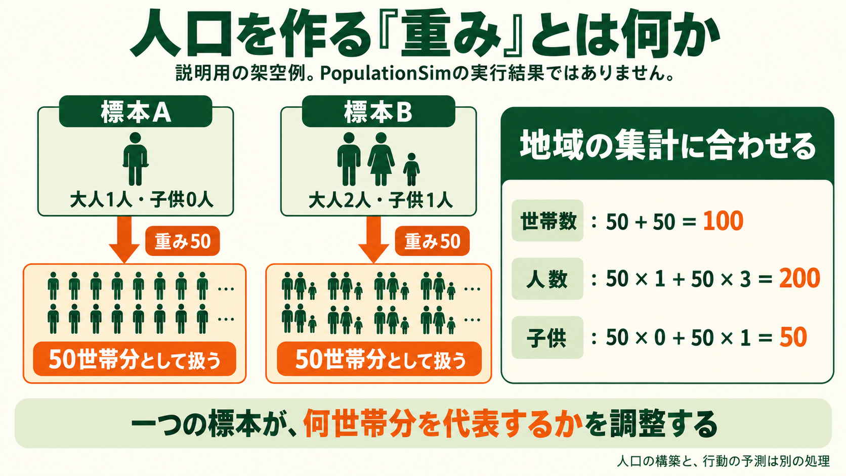
Illustration with Japanese labels.

populationsim/steps/initial_seed_balancing.py reads settings and controls and passes them to balancing. ListBalancer.balance in populationsim/balancing/single_balancer.py handles initial weights, targets, bounds, and importance, and returns convergence information, final weights, and target-versus-achieved control totals. The code can relax constraints; do not assume all targets always match exactly.

populationsim/steps/integerize_final_seed_weights.py passes floating-point weights and targets to integerization. Household and person totals must be checked again afterward. This is not simply equivalent to rounding each weight.

B17001, used for our initial population component, is an aggregate table, not PopulationSim’s entire required input. A six-cell reconstruction and PopulationSim’s household–person sample synthesis operate at different levels. Household modeling requires corresponding household and person inputs.

SFT inputs and calculation

Supervised fine-tuning, or SFT, uses examples pairing an input x with an answer y. For human response prediction, x might contain attributes, experimental conditions, and a question; y might be the observed answer.

A language model turns text into tokens and computes each answer token’s probability conditional on earlier tokens. The probability of the whole answer is their product. SFT generally minimizes the answer’s negative log probability. In a one-answer teaching example, probability 0.2 gives loss about 1.609; probability 0.8 gives about 0.223.

loss = −log(probability of the example answer)

Gradients calculate how the loss depends on settings, and an optimizer updates them. Some methods update all weights; others train a small set of added parameters. “SFT” alone does not specify which parameters were updated.

Using someone’s observed answer as a training example is not the same as knowing their universally correct answer. Responses can vary even under the same conditions, so evaluate both individual predictions and population distributions.

DPO inputs and calculation

Direct Preference Optimization, or DPO, uses one input x, a comparatively chosen answer y+, and a comparison answer y−. A fixed reference model and the model being trained both assign probabilities to the answers.

Conceptually, compare:

trained model’s chosen/comparison probability ratio
÷ reference model’s chosen/comparison probability ratio

For illustration, let the reference probabilities be 0.3 and 0.7, and the trained model’s probabilities 0.6 and 0.4. The ratio of ratios is (0.6/0.4)/(0.3/0.7) = 3.5: the chosen answer’s relative probability increased compared with the reference.

The original loss takes the logarithm of this ratio, multiplies by β, applies the sigmoid σ, and averages the negative log result. With β = 1, a ratio of 1 gives approximately 0.693 loss; 3.5 gives approximately 0.251. This simple example uses whole-answer probabilities; language-model training requires token-level calculations.

L_DPO = mean[−log σ(β × log(ratio of ratios))]

In the original formulation, β controls the relationship with the reference policy. Do not read it as simply “larger means weaker constraints.” First understand the fixed reference and answer comparison, then inspect the paper’s equation and implementation settings.

Socrates describes contrasting different answers given by different people under the same experimental condition, placing the matched person’s actual answer on the chosen side. The meaning of those labels differs from DPO that learns general preferences about prose.

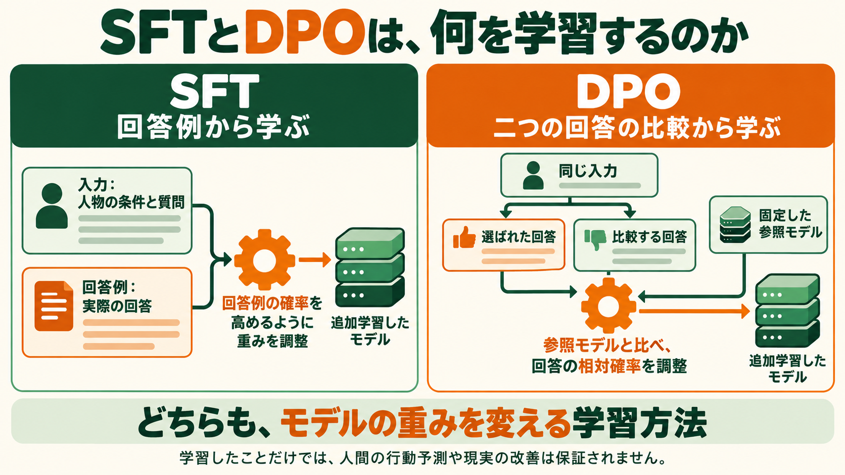
Japanese labels.

Reading the code

For PopulationSim, read controls, samples, the contribution table, balancing, integerization, and error checks in that order. For Socrates, inspect people, conditions, answers, splits, model settings, and the paper’s SFT/DPO sections. Then read LLaMA-Factory’s src/llamafactory/train/sft/workflow.py and src/llamafactory/train/dpo/workflow.py to see where models and data enter training.

Dependencies were not installed, models were not trained or run, and PopulationSim was not executed for this explainer. Illustrative calculations are separate from reading public code.

Sources

• PopulationSim
• Socrates paper
• Original DPO paper
• InstructGPT paper
• LLaMA-Factory

Learning draft, October 12, 2026.