Generating populations with diffusion models: separate training from sampling

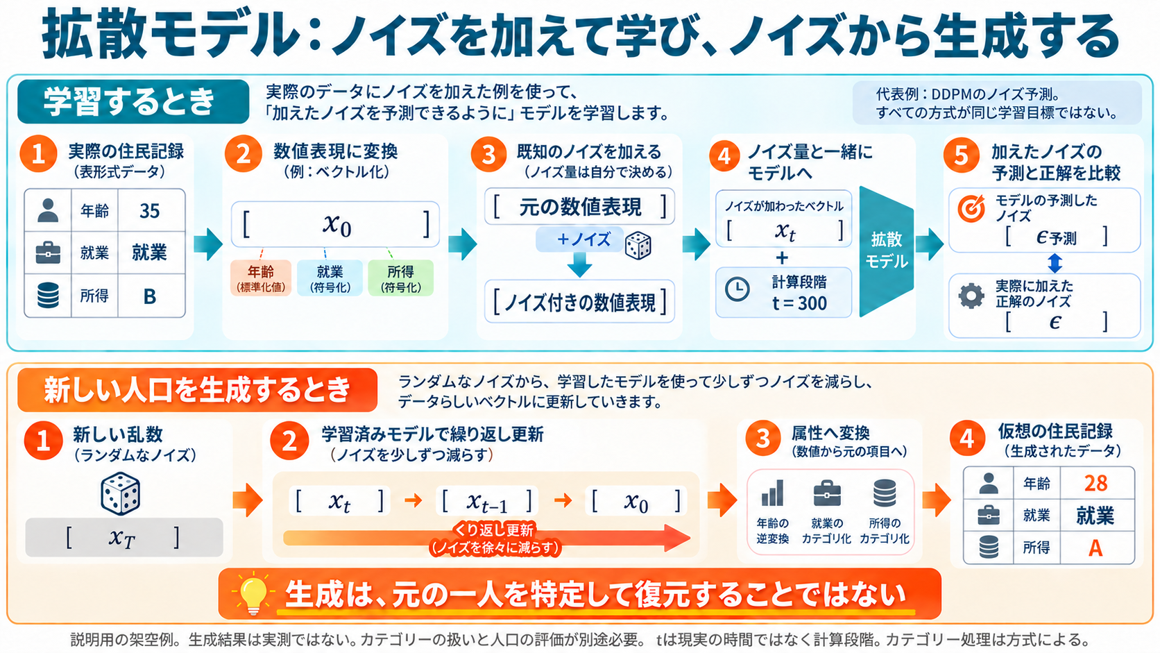
Japanese labels. Distinguishing DDPM, TabDDPM, latent diffusion, and population-synthesis code reveals different learning targets and generation procedures.

The objective

As with Bayesian networks, VAEs, and GANs, we want synthetic resident records. Diffusion models learn updates that bring corrupted representations toward the data distribution. Training uses observations; generation starts with fresh randomness. It does not search for and restore a particular original resident.

1. What noise means

Noise here means random numerical variation. Attributes first need numerical representations: standardized age, for example, is not age in years. Randomness is mixed into that representation by a specified rule. This manipulates data, not people.

Adding static to a photo is a useful analogy, but population records are not photographs. Categorical employment status cannot automatically receive the same operation as numerical age.

2. DDPM training

Ho, Jain, and Abbeel’s Denoising Diffusion Probabilistic Models provides one foundational example. Algorithm 1 selects an observed record, a noise level, and known noise, then trains the model to predict that noise by minimizing squared prediction error.[1]

The model can receive an entire attribute combination, letting other fields help with a noisy field. Whether it learned useful relationships still needs testing.

Because we generated the added noise, its value is known; no person must manually label every noisy example. Observed records are still required. This does not let a model discover the true population without data.

The index t denotes a computational noise stage, not tomorrow or next year. Training can directly compute the selected noisy stage without running every preceding stage.

3. Following one number

Consider a stage mixing original value x0 with coefficient 0.8 and standard-normal noise epsilon with coefficient 0.6. Their squared coefficients sum to one.

If x0 = 2.0 and epsilon = −1.0, the noisy value is 0.8 * 2.0 + 0.6 * (-1.0) = 1.0. An exact noise estimate lets us algebraically recover 2.0. If predicted noise is −0.5, estimated x0 is 1.625.

But observing an unknown noisy value of 1.0 does not uniquely identify its original as 2.0. Training learns distributionally plausible updates across many examples. This known-noise calculation checks an equation, not a trained denoiser’s performance.

4. Sampling a new record

Start from fresh noise and repeatedly apply a trained model. DDPM uses estimated noise, stage-dependent coefficients, and randomness when appropriate to calculate the next state. It is not a single subtraction of predicted noise. Finally decode the representation into attributes.

This creates a new synthetic record, not a return to an observed 35-year-old. Different randomness can produce different records; diversity and distributional accuracy require separate evaluation.

5. Categorical attributes

TabDDPM’s 2023 paper combines Gaussian diffusion for numerical variables with multinomial diffusion for categories. Categorical corruption probabilistically perturbs values across categories, while the learned reverse process can use other attributes.[2]

TabSyn instead represents mixed-type attributes in a latent space, performs diffusion there, and decodes them. VAE and diffusion are not necessarily competing categories. We checked its abstract and author repository, not a complete reproduction.[3]

6. What population-synthesis code actually does

We read a fixed version of Darsel and colleagues’ public repository. models/Diffusion/Diffusion_Embedded_data/train_Diffusion_Embedded_Data.py trains on embedded data. Model_Diffusion.forward in model_Diffusion.py calls EDMLoss.

In utils/utils_diffusion.py, EDMLoss.__call__ chooses sigma, generates noise n, and computes denoise_fn(y + n, sigma). Its target is original data y, not noise n, using weighted squared error. It should not be described identically to DDPM noise prediction.

The same file’s sample starts with new normal noise and repeats sample_step. Updates use model estimates and stage-dependent step sizes, with a second-order correction except at the final step. sample_Diffusion_Embedded_Data.py saves outputs. Methods differ in stage counts and reverse-update equations.[4]

7. Strengths and limits

Diffusion decomposes generation into learned denoising updates without requiring the standard GAN’s G/D competition. It is not a universal solution to mode collapse: rare-group omission, training bias, and constraint violations still need checking. Compare the cost of iterative sampling too.

Darsel and colleagues’ 2026 comparison found Bayesian networks strong in its 12-attribute setting and diffusion promising among deep models. This makes diffusion a candidate whose added value should be measured with a shared evaluator, not a universal winner.[5]

8. Scope of this explainer

We read papers and code and checked noise-mixing and known-noise reconstruction equations. We did not train or run a diffusion network, generate a real population, or reproduce paper performance.

For LLM comparisons, separate fine-tuning on serialized microdata from prompting with public aggregates. Household structure and comparisons against real evidence are additional requirements.

Sources

1. Ho, Jain, Abbeel, DDPM, 2020: methods and training/sampling algorithms.
2. Kotelnikov et al., TabDDPM, ICML 2023: sections 3–4.
3. Mixed-Type Tabular Data Synthesis with Score-based Diffusion in Latent Space; author code. Abstract and architecture checked here.
4. PopulationSynthesis public code: main operations inspected.
5. 2026 comparison: final-version methods, results, and limitations checked in the preceding lesson.