Bayesian networks: connecting conditional probabilities to generate a population

A Bayesian network represents the joint distribution of several attributes using a directed graph and conditional probability tables. It extends a statement such as “30% of boys cycle to school” into a model that can generate synthetic people with several attributes.

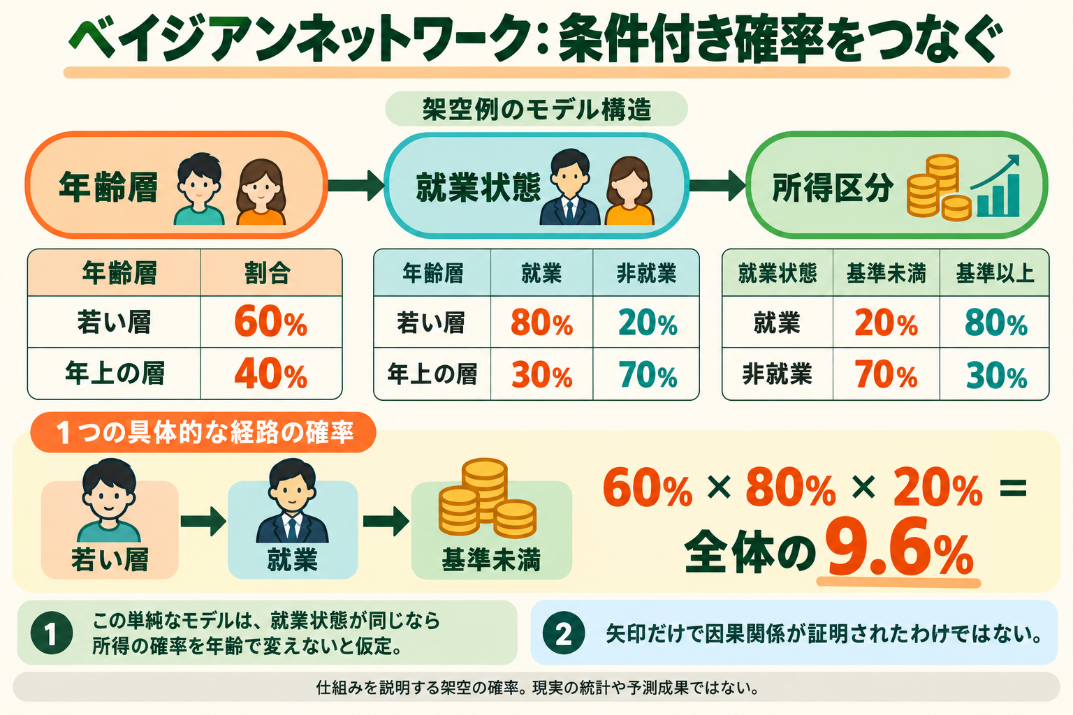
Illustrations in this article have Japanese labels.

Both a graph and probability tables

Our teaching structure is age group → employment → income category. Circles or boxes are nodes; arrows are edges. An arrow’s source is a parent of its destination. During generation, choose parents first and sample children from the table corresponding to their parents’ values.

All probabilities here are fictional: 60% younger and 40% older; employment probability 80% for younger people and 30% for older people; below-threshold income probability 20% if employed and 70% otherwise. The remaining probability goes to the other category.

To generate a person, first sample age group using 60%. If younger, use employment probability 80%. If employed, use below-threshold income probability 20%. Draw a separate random number at each step for each person.

Probability of a combination

The probability of younger, employed, and below threshold is 0.60 × 0.80 × 0.20 = 0.096, or 9.6%. Among 100 independently generated people, its expected count is 9.6—not a claim that a particular draw produces a fractional person.

P(age, employment, income)
 = P(age) × P(employment | age) × P(income | employment)

This factorization corresponds to our graph. For three arbitrary variables, the final term would be P(income | age, employment). Dropping age requires an assumption: within an employment category, this model does not change income probabilities by age. If that assumption is unsuitable, add age → income and estimate a table conditional on both age and employment.

A model therefore specifies omitted relationships as well as drawn arrows. Bayesian networks use directed acyclic graphs (DAGs), which contain no directed path returning to its starting node.

Where structure and probabilities come from

We chose them manually for teaching. In research, distinguish structure learning—choosing connections—from parameter learning—estimating probability tables for a chosen graph.

If 80 of 100 sampled younger people are employed, the simple frequency estimate is 80%. Sampling weights, small groups, unobserved parent combinations, and geographic transfer still matter. More parents require more condition-specific data, so adding edges is not automatically better.

Sun and Erath’s 2015 study used Singapore’s HITS2012 survey as a reference population and compared synthesis from smaller samples. It searched structures using bnlearn’s tabu search, learned structure and probabilities, and generated records. Input information differed from the IPF comparison, so a score is not evidence of superiority in all settings. The reference was a survey dataset, not individual records for every Singapore resident.[1]

Sampling in public code

We read pgmpy’s BayesianModelSampling.forward_sample. It processes parents before children, obtains probability tables with get_cpds, selects conditions using previously sampled parent values, and samples. A root node uses its unconditional probabilities.[2]

We did not run pgmpy. A short Python standard-library lesson implemented the same three-stage idea, checked that the eight combination probabilities sum to one and the specified path has probability 9.6%, and sampled 10,000 fictional records. This was not real-data training or replication of the paper’s scores.

Dependence is not intervention

These arrows express probabilistic dependencies. An observed income distribution among employed people does not establish how income would change if someone were given employment. Prediction and intervention are different questions.

For Manager, Bayesian networks are one candidate for population synthesis. We must separately evaluate supplied geographic totals and held-out combinations. There is no evidence that Aaru or Simile uses this particular network.

[1] Sun and Erath, A Bayesian network approach for population synthesis. Sections 3.1–3.3 and the experimental setup were checked.

[2] pgmpy public source. We read the public development source; this is not an independent performance evaluation.

Conditional probability is a component, not the whole network

A conditional probability is a quantity such as employment probability given younger age. A Bayesian network combines a graph with its probability tables to represent a joint distribution. The components and their arrangement are not interchangeable terms.

IPF, Bayesian networks, and LLMs are representative examples selected for this course, not the field’s only methods or an established market top three. They also sit at different conceptual levels: IPF is an adjustment algorithm, a Bayesian network is a probabilistic model, and LLMs are a family of models. Generative models such as VAEs and combinatorial optimization also exist; methods can be combined.

IPF is the method; ipfn is a Python library implementing it.

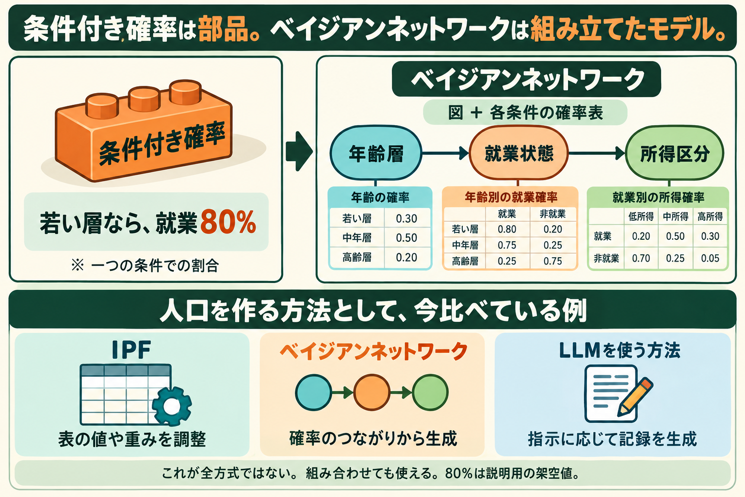
The supplementary figure uses fictional probabilities and a separate example from the two-age-group lesson. It illustrates the relationship between components and a complete model.